If you work in data analysis, data science, or science communication, your use of data visualizations can make or break the take home message. However, it may not be technically obvious how to do this. In the past, I’ve used Microsoft Excel to export a chart as a PDF file and then work with it in Adobe Illustrator to produce a final product. But if you want to do this with R, RStudio, and Inkscape here is one way to produce infographics.
Process and Understand Your Data
Before you can communicate your findings or insights, you must understand your data. In the R Tidyverse, the data science project follows these steps:
- Import
- Tidy
- Understand (Transform, Visualize, and Model)
- Communicate
For the sake of time, we’re going to skip ahead to the fourth step, Communicate. I’m going to assume you can handle steps 1-3 on your own. In this example, I’m using R version 4.3.3 and RStudio version 2024.04.2. This is sample data I used for this project.
# R package libraries used ####
library(tidyverse)
library(janitor)
library(scales)

# sample data ####
my_data <- structure(list(q1 = c(
  "forensic scientist", "procurement", "archaeologist",
  "archaeologist", "real estate", "psychologist", "museums", "anthropologist",
  "psychologist", "ultrasound technician", "business consultant",
  "teacher", "archaeologist", "historian", "psychologist", "counselor",
  "librarian", "engineer", "exploring opportunities", "forensic scientist",
  "procurement", "librarian", "engineer", "meteoroligist", "engineer",
  "engineer", "business management", "engineer", "business", "actuary",
  "engineer", "entrepreneur", "sonographer", "lawyer", "librarian",
  "cultural ambassador", "engineer", "psychologist", "public relations manager",
  "cultural ambassador", "entrepreneur", "ultrasound technician",
  "entrepreneur", "accountant", "athletic director", "professional athlete",
  "market researcher", "real estate", "tour guide", "media production",
  "environmentalist", "manufacturing", "physical therapist", "radiology technician",
  "social worker", "environmentalist", "architect", "engineer",
  "physical therapist", "exploring opportunities", "athletic trainer",
  "engineer"
), q2 = c(
  "interested in human bones", "teacher", "archaeologist",
  "archaeologist", "teacher", "journalist", "archaeologist", "archaeologist",
  "historian", "lawyer", "business consultant", "librarian", "archaeologist",
  "archaeologist", "journalist", "social worker", "librarian",
  "advertising executive", "political consultant", "archaeologist",
  "teacher", "librarian", "digital marketing specialist", "controller",
  "lawyer", "architect", "business consultant", "engineer", "business consultant",
  "business consultant", "market researcher", "business consultant",
  "sonographer", "lawyer", "librarian", "cultural ambassador",
  "engineer", "social worker", "public relations manager", "cultural ambassador",
  "business consultant", "health and wellness manager", "business consultant",
  "lawyer", "health and wellness manager", "lawyer", "market researcher",
  "health and wellness manager", "tour guide", "journalist", "public relations officer",
  "teacher", "health and wellness manager", "health and wellness manager",
  "social worker", "public relations officer", "health and wellness manager",
  "advertising executive", "journalist", "journalist", "tour guide",
  "journalist"
), course = c(
  "ASB 102", "ASB 102", "ASB 102", "ASB 102",
  "ASB 102", "ASB 102", "ASB 102", "ASB 102", "ASB 102", "ASB 102",
  "ASB 102", "ASB 102", "ASB 102", "ASB 102", "ASB 102", "ASB 102",
  "ASB 102", "ASB 102", "ASB 102", "ASB 102", "ASB 223", "ASB 223",
  "ASB 223", "ASB 223", "ASB 223", "ASB 223", "ASB 223", "ASB 223",
  "ASB 223", "ASB 223", "ASB 223", "ASB 223", "ASB 223", "ASB 223",
  "ASB 223", "ASB 223", "ASB 223", "ASB 223", "ASB 223", "ASB 223",
  "ASB 223", "ASB 223", "ASB 252", "ASB 252", "ASB 252", "ASB 252",
  "ASB 252", "ASB 252", "ASB 252", "ASB 252", "ASB 252", "ASB 252",
  "ASB 252", "ASB 252", "ASB 252", "ASB 252", "ASB 252", "ASB 252",
  "ASB 252", "ASB 252", "ASB 252", "ASB 252"
), q1_lump = structure(c(
  6L,
  6L, 1L, 1L, 6L, 5L, 6L, 6L, 5L, 6L, 6L, 6L, 1L, 6L, 5L, 6L, 4L,
  2L, 6L, 6L, 6L, 4L, 2L, 6L, 2L, 2L, 6L, 2L, 6L, 6L, 2L, 3L, 6L,
  6L, 4L, 6L, 2L, 5L, 6L, 6L, 3L, 6L, 3L, 6L, 6L, 6L, 6L, 6L, 6L,
  6L, 6L, 6L, 6L, 6L, 6L, 6L, 6L, 2L, 6L, 6L, 6L, 2L
), levels = c(
  "archaeologist",
  "engineer", "entrepreneur", "librarian", "psychologist", "Something else"
), class = "factor"), q2_lump = structure(c(
  5L, 5L, 1L, 1L, 5L,
  4L, 1L, 1L, 5L, 5L, 2L, 5L, 1L, 1L, 4L, 5L, 5L, 5L, 5L, 1L, 5L,
  5L, 5L, 5L, 5L, 5L, 2L, 5L, 2L, 2L, 5L, 2L, 5L, 5L, 5L, 5L, 5L,
  5L, 5L, 5L, 2L, 3L, 2L, 5L, 3L, 5L, 5L, 3L, 5L, 4L, 5L, 5L, 3L,
  3L, 5L, 5L, 3L, 5L, 4L, 4L, 5L, 4L
), levels = c(
  "archaeologist",
  "business consultant", "health and wellness manager", "journalist",
  "Something else"
), class = "factor")), row.names = c(NA, -62L), class = c("tbl_df", "tbl", "data.frame"))
Use ggplot2 to Create Your Charts
“ggplot2 is a system for declaratively creating graphics.”
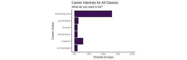
After using the janitor R package to create summary tables we’re going to use the ggplot2 R package to create our charts. Here’s the code and resulting charts:
 |
|---|
| The code block below produces the above chart as a 10.2in x 3.26in image. |
my_data %>%
  tabyl(q1_lump) %>% # janitor produces a data table
  ggplot() +
  geom_col(
    mapping = aes(x = q1_lump, y = percent),
    fill = "#3D1255", # color doesn't matter as much Inkscape can update it
    color = "black",
    width = 1) +
  coord_flip() +
  scale_y_continuous(
    labels = label_percent(), # use of the scales R package
    limits = c(0, 1)) +
  labs(
    title = "Career Interests for All Classes",
    subtitle = "What do you want to be?",
    x = "Career choice",
    y = "Percent of class") +
  theme_classic() +
  theme(aspect.ratio = 2/3) #

ggsave(filename = "chart-example-01.png") # Saved as a 10.2in x 3.26in image
Notice that if we copy and paste the image to Inkscape (version 1.2.2), the png file is a raster, and we are unable to easily edit individual elements. There is a bunch of white space on both the left and right edges of the image. This means we should update our use of ggsave to specify format (device = “svg”), dimensions, and scale.
ggsave(
  filename = "chart-example-01.svg",
  device = "svg",
  width = 75,
  height = 50,
  units = "mm",
  scale = 1.75
)
Inkscape
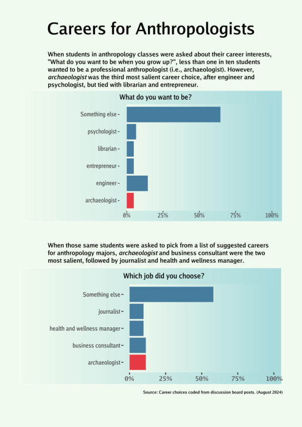
Use Inkscape to import the SVG created in RStudio. Use Inkscape to make tweaks to the charts themselves, like updating the color for one of the bars to call attention to it. But from here I seek to transform the charts to an informational graphic.
 |
|---|
| This is the final product, an informational graphic. |
One of the things you may notice when exporting graphics from RStudio (with ggplot2 and ggsave) is that it can be challenging to export charts with consistent sizes and scales. Unfortunately, I don’t have a good solution for this. However, some Mastodon users had the following suggestions when I asked for advice:
- RAWGraphs 2.0
- Cartographic symbol generator
- Save as a PDF. Work with the PDF in Inkscape.
- Try Matplotlib